Cumulative Distribution Function (CDF)
Let us consider a random variable X with a probability distribution given by $P(x)$.
The Cumulative Distribution Function F(x) for a given value X=x is given by the probability of
obtaining a X value less than or equal to x:
\(~~~~~~~~~~~~~~~~~~~~~ F(x)~=~P(X \leq x) \)
If P(x) is the probability distribution of a discrete variable X with possible values in the range $[x_{min}, ~x_{max}]$, then the CDF is given by
\(~~~~~~~~~~~~~~~~~~~~~F(x)~=~\displaystyle \sum_{x_{min}}^{x_{max}} P(x) \)
For a continuous variable X with a Probability Density Function $P(x)$ defined in the range $[x_{min}, ~x_{max}]$, the Cumulative Distribution Function $F(x)$ is
obtained by integration:
\(~~~~~~~~~~~~~~~~~~~~~G(x)~=~\displaystyle \int_{x_{min}}^{x_{max}} P(x) dx ~~~~~~ \)
Example 1: The Cumulative Density Function for a Poisson distribution with mean $\mu$ is given by $~~F(x)~=~\displaystyle \sum_{X=0}^{x} \dfrac{\mu^X e^{-\mu}}{X!}$
Example 2: The cumulative Distribution Function of a Gaussian distribution is given by
$~~F(x)~=\displaystyle \int_{-\infty}^{x} \dfrac{\large{e}^{-z^2/2}}{\sqrt{2\pi}} dz$
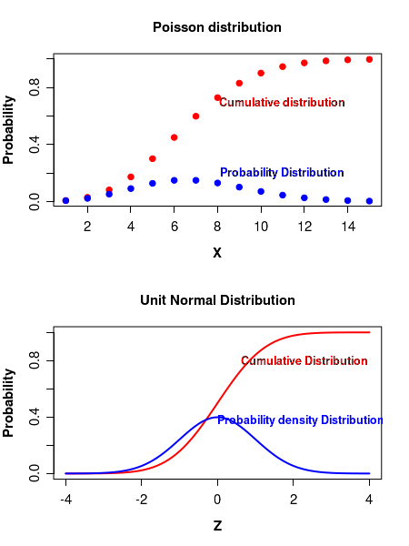
The Figure-1 below displays the cumulative probability distributions for a Poisson distribution (with a
mean value of 7) and a unit normal distribution. As expected, the cumulative PDF has the typical 'S' shape
satirating at the maximum probability of 1 in both the cases.
The R script for plotting the above distributions is as follows:
## Plotting the cumulative distribution function for Poisson distribution

x_pois = seq(1,15)

mu_pois = 7  # mean of Poisson distribution

probs_pois = dpois(x_pois,mu_pois)

cumulative_pois = ppois(x_pois,mu_pois) ## computes the cumulative distribution

plot(x_pois, cumulative_pois, pch=19, col="red",xlab="X", ylab="Probability",
      font.lab=2, cex.lab=1.2, main="Poisson distribution", cex.axis=1.2)
lines(x_pois, probs_pois, type="p", col="blue", pch=19)
text(11, 0.7, "Cumulative distribution", col="red", font=2)
text(11, 0.2, "Probability Distribution", col="blue", font=2)


## Plotting the cumulative distribution function for unit normal distribution

Z_norm = seq(-4,4,0.1)

probs_norm = dnorm(Z_norm)

cumulative_norm = pnorm(Z_norm) ## computes the cumulative distirbution.

plot(Z_norm, cumulative_norm, , xlab="Z", ylab="Probability", type="l", lwd=2, col="red",
     main="Unit Normal Distribution", font.lab=2, cex.lab=1.2, cex.axis=1.2)
lines(Z_norm, probs_norm, type="l", col="blue", lwd=2)
text(2.3, 0.8, "Cumulative Distribution", col="red", font=2)
text(2.2, 0.37, "Probability density Distribution", col="blue", font=2)
The empirical Cumulative Distribution Function (empirical CDF)
The empirical Cumulative Distribution Function (empitrical CDF) is the Cumulative Distribution Function computed
for a given
sample data.
For a given sample data set, the empirical cumulative probability at any
possible value x is the fraction obtained by dividing the cumulative frequency upto x by the total frequency of the data.
Alternatelly, we can sort the data in ascending order and obtain the cumulative probability at each $x_i$ by dividing the
order of $x_i$ by the total number of data points.
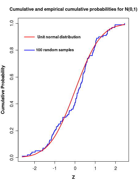
The Figure-2 below shows the empirical cumulative probability distribution of 100 data points randomly drawn from
a unit normal distribution. For comparison, the PDF of unit normal distribution is plotted as solid curves in the data.
In the above figure, we observe that the empirical CDF of sample data follows the original PDF approximately.
The deviations can be severe for small sample sizes or when we compare th CDF of our data with a wrong distribution.
If we draw another set of 100 random points, the empirical CDF will look different from the above one due to
random fluctuations.
The R script for plotting the above distributions is as follows:
## plotting cumulative and empirical distributions for unit gaussian

set.seed(1237)  # set the seed for random number generator
                # (to reporduce sample result in every run)

## generate 100 random deviates from unit normal distribution
Z = rnorm(100)

## sort the data points
Z = sort(Z)

## cumulative probabilities for sorted Z values. Empirical cdf
empirical_cdf = seq(1,length(Z))/length(Z)   ## cumulative Z

## this is the cumulative probabilities of theoretical
##    unit normal distribution for every Z value

cumulative = pnorm(Z)

## plot Z values against empirical probabilities as step lines
plot(Z, empirical_cdf, type="s", col="blue", ylab="Cumulative Probability", lwd=2,
     main="Cumulative and empirical cumulative probabilities for N(0,1)",
           font.lab=2, cex.lab=1.2, cex.axis=1.2)

# add the cumulative probabilities od unit normal as lines.
lines(Z, cumulative, type="l", col="red", lwd=2)

segments(-2.5, 0.9, -2.0, 0.9, col="red", lwd=2)
text(-0.8, 0.9,"Unit normal distribution", font=2)

segments(-2.5, 0.8, -2.0, 0.8, col="blue", lwd=2)
text(-1.0, 0.8,"100 random samples", font=2)