CountBio
Mathematical tools for natural sciences
Biostatistics with R
Estimation of uncertainities using function derivatives
On many occasions, we find that a quantity (say) \(\small{f}\) is epxressed as a function of another quantity, say \(\small{x}\). In the language of mathematics, \(\small{x}\) is an independent variable and \(\small{f}\) i>s a function of x written symbolically as \(\small{f(x)}\). The function f(x) can have any form, from simple straight line relationship to very complicated formula. We will consider a simple exponential relationship of the form, \(~~~~~~~~~~~~~~~~~~~~~~~~~~~~~\small{f(x) = 13.6 e^{1.2x}~~}\) Now suppose we do an experiment and determine the value of \(\small{x}\) to be 0.96 with an uncertainity (error) of 0.12. We can find the value of f at x = 0.96 by substituting it in the above formula. We get \(\small{y = 13.6 e^{1.2\times0.96} = 43.04}\). That is fine. But, given an uncertainity of 0.12 on the x value of 0.96, what is the uncertainity on the computed value 43.04 of y? . We need to use the idea of "total differential" from calculus compute this error propagation from x to its function f(x) .
Absolute and relative changes
Consider a increment in the value of x by a small value \(\small{\Delta x }\). The value of function f at these two points is \(\small{f(x)}\) and \(\small{f(x + \Delta x) }\). Then, \(~~\small{\Delta f = f(x + \Delta x) - f(\Delta x) }\) is the absolute change in f for a change \(\small{\Delta x }\) in x. \(\small{~~~~\dfrac{\Delta f}{f}~~ }\) is the corresponding relative change in f. \(\small{~~~~\dfrac{\Delta f}{f} \times 100 \%~~~ }\) is the corresponding percentage change in f.
The derivative of a function at a given point
Consider the two points \(\small{P(x, f(x)) }\) and \(\small{Q(x + \Delta x, f(x + \Delta x) }\) on the curve f(x). See the figure below:
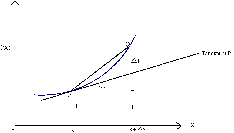
An increment of \(\small{\Delta x }\) on x creates a change of \(\small{\Delta f }\) in f. As the increment \(\small{\Delta x }\) becomes smaller and smaller, the two points \(\small{P(x, f(x) )}\) and \(\small{Q(x+\Delta x, f(x+\Delta x)) }\) come closer and closer, and in the limit when \(\small{\Delta x }\) approaches zero, the chord joining the points P and Q will become the tangent to the curve at the point \(\small{(x, f(x))}\). In this limit, the ratio \(\small{\dfrac{\Delta f}{\Delta x} }\) which represents the change in f for a unit change in x becomes a constant, and is equal to the slope of the tangent to the curve at x. We write this as, $$ \small{ \lim_{\Delta x\to 0} \dfrac{\Delta f}{\Delta x} = \lim_{\Delta x\to 0} \dfrac{f(x+\Delta x) - f(x)}{\Delta x} = m = slope~of~the~tangent~at~x}$$
The slopes of tangent at various values of x are different. It is a continuous function of x, since f(x) is a continuous function. Therefore, we can find represent the slope of tangent at various x values as another function, called derivative function , represented by \(\small{f'(x)}\). Once this derivative function is found, slope of tangent at any point x=a will be just \(\small{f'(a) }\). In our calculus class, have learnt to compute the derivative function \(\small{f'(x)}\) for any continuous function \(\small{f(x)}\). The derivative f'(a) at x=1 gives the instantaneous rate of change of f with respect to x at x=a. It is a slope of the tangent for the curve f(x) at x=a, and is a number.
The differential of a function
For a small change \(\small{\Delta x}\) along on x, the function f(x) changed by \(\small{\Delta f }\). The ratio \(\small{\dfrac{\Delta f}{\Delta x} }\) gives the derivative (or slope of tangent) at x in the limit when \(\small{\Delta x }\) tends to zero. This "\(\small{\Delta x }\) tends to zero" is a mathematical concept. In real life situations, we are interested in computing the change in f for a very small, but finite change in x . This change can be as small as we require, but will not "tend to zero" as a limit. Let \(\small{dx }\) be a very small change in \(\small{x}\). Let us denote the corresponding change in \(\small{f}\) by \(\small{df}\). In order to find a relationship between \(\small{dx}\) and \(\small{df}\), we make use of the tangent to the curve at \(\small{x}\). See the figure below:
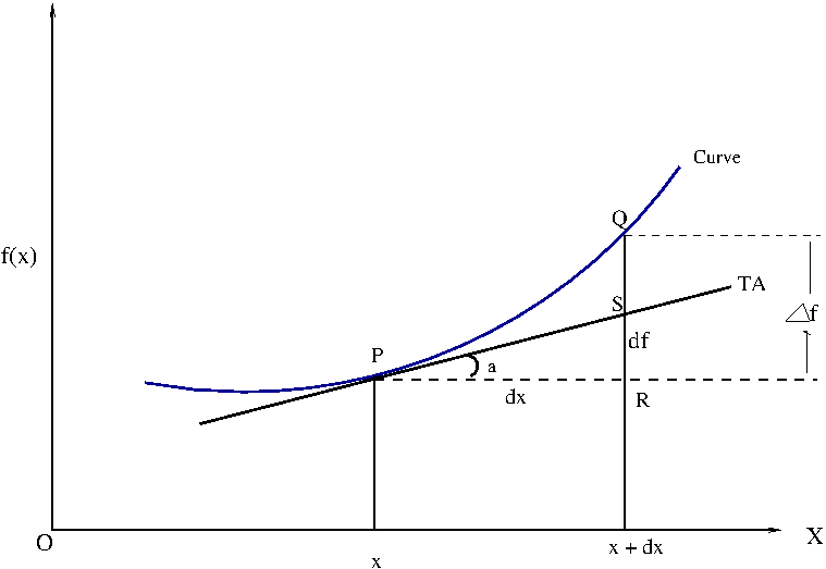
In the figure above, TA is the tangent line to the curve at a point \(\small{x}\), whose slope at \(\small{x}\) is \(\small{f'(x)}\).
When \(\small{x}\) incremented by an amount \(\small{dx}\), there is a vertical increment of \(\small{df}\)
along the tangent line, while the vertical increment along the curve is \(\small{\Delta y }\).
The difference \(\small{\epsilon = \Delta f - df }\) between the climb along the curve and the tangent reduces as the increment \(\small{dx }\) becomes smaller and smaller. We now have a freedom to choose \(\small{\Delta x }\) sufficiently small so that this error \(\small{\epsilon }\) becomes negligible when compared to the dimensions of the problem..
The, we can write, for the right angled triangle PRS,
\(\small{ tan(a)~ = ~\dfrac{SR}{PR} ~= ~\dfrac{df}{dx}~ =~ f'(x)~ =~ slope~of~the~tangent~at~x }\)
From this, we get this important result:
The differential of a function with many variables
We have a function that depends on more than one variable, uncertinities in each one of these variables contribute to the uncertainity in the function. The differential of the function has contrinution from the variations in all its variables. The differential of a single variable function \(\small{f(x) }\) is given by \(\small{df = f'(x)dx}\). Suppose the function f is dependent on three variables \(\small{x,y,x}\). In this case, the above concept is extended to write the total differential of f in terms of the partial derivatives of f with respect to its variables as, \(~~~~~~~~~~~~\small{df~=~\dfrac{\partial f}{\partial x} dx~+~\dfrac{\partial f}{\partial y} dy~+~\dfrac{\partial f}{\partial z} dz }\) Where, \(~~\small{\dfrac{\partial f}{\partial x} }~~\), \(~~\small{\dfrac{\partial f}{\partial y} }~~\) and \(~~\small{\dfrac{\partial f}{\partial z} }~~\) represent the partial derivative of the function f with respect to the variables x, y and z respectively and ther terms dx, dy and dz represent the increment in the respective variables. To take a partial derivative of the function with respect to any one variable, differentiate the function with respect to that variable, while treating the remaining variables as constants. As an example, we take the partial derivatives of the function \(~~\small{f = x^2y^2z^2 }\) as follows: \(~~~~~~~~~\small{\dfrac{\partial f}{\partial x} = 2x(y^2z^2) }~~~~~~\) (differential the x term, keep y and z as constants) \(~~~~~~~~~\small{\dfrac{\partial f}{\partial y} = 2y(x^2z^2) }~~~~~~\) (differential the y term, keep x and z as constants) \(~~~~~~~~~\small{\dfrac{\partial f}{\partial z} = 2z(x^2y^2) }~~~~~~\) (differential the z term, keep x and y as constants)