CountBio
Mathematical tools for natural sciences
Basic Statistics with R
Hypergeometric distribution
In the binomial distribution, it is assumed that the probability \(p\) for success remains the same for the \(n\) trials. This can be achieved in two ways:
- The population from which samples are drawn is infinite or so large that while sampling \(n\) events(trials) one by one, the population size does not change enough to alter the probability \(p\) between the trials.
- The population size is finite, but the sampling is done with replacement so that the probability \(p\) remains the same for the \(n\) trials.
The hypergeometric distribution applies to sampling without replacement from a finite population consisting of dual outcomes. Since the population is finite, drawing a sample withour replacement changes the population and hence alters the probability \(p\) between successive trials.
We will derive an expression for hypergeometric probability \(\small{P(x,n,N_1,N_2)}\) of getting \(x\) successes out of \(n\) trials from a population consisting of \(N_1\) successes and \(N_2\) failures.
Derivation of hypergeometric probability distribution: Suppose a list of students contains names of \(\small{N_1}\) girls and \(\small{N_2}\) boys. Let \(\small{N=N1+N2}\) be the total population. Assume that the success is defined as randomly picking the name of a girl from this list. Let us select a random sample of size \(n\) from the list and \(x\) be the number of girls (successes) among the \(n\) names. If the sampling is done one at a time with replacement, the distribution of x is a binomial \(\small{P_b(x, n, p)}\) where \(\small{p = \frac{N_1}{N_1+N_2} }\) . However, if the sampling of n names is done without replacement, the probability p changes during every draw. So, the distribution of \(x\) is not binomial. In this case, we compute the probability \(P(x)\) that \(x\) out of \(n\) selected students will be girls as ratio of number of possibilities: \( \small{ P(x) = \dfrac{number~of~ways~x~successes~occur \times number~of~ways~(n-x)~failures~occur}{total~number~of~selections}} \) From the information given above, \(x\) successes can occur in \(~\small{_{N_1}C_x~}\) ways and \(\small{(n-x)}\) failures can occur in \(~\small{_{N_2}C_{n-x}~}\) ways. The total number of ways we can draw n objects out of \(\small{N=N_1+N_2}\) objects is \(\small{_{N_1+N_2}C_n}\) With this, we get the hypergeometric distribution given by, \( \small{P_h(x,n,N_1,N) = \dfrac{_{N_1}C_x~\times~ _{N_2}C_{n-x}}{_{N_1+N_2}C_n} = \dfrac{_{N_1}C_x ~\times~ _{N-N_1}C_{n-x}}{_{N}C_n}} \)
.
To summarize, the hypergeometric probability \(\small{P(x,n,N_1,N)}\) of getting \(x\) successes out of \(n\) draws without replacement from a population consisting of \(\small{N_1}\) successes and \(\small{N-N_1}\) failures is given by,
In the above formula, \(x\) is a non-negative integer such that \(x \le n \), \(~x\small{ \le N_1}~\) and \(~\small{n-x \le N_2.} \)
When \( \small{n \ll (N_1 + N_2)} \), the probability values of the hypergeometric distribution are closer to the binomial probabilities.
Why the name "hypergeometric distribution"?
The hypergeometric distribution derives its names from the resemblence of its density distribution formula to the hypergeometric identity given by, \( \small{_{a+b}C_r = \sum\limits_{k=0}^r {_aC_k} \times {_bC_{r-k}} }\)
The mean and variance of the hypergeometric distribution
The expressions for the mean and the variance of the hypergeometric distributions are given by (derivation not shown),
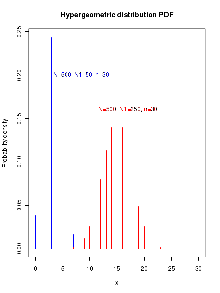
The plot of hypergeometric probability distribution
The plot of hypergeometric probability for various values of the parameters are shown in the figure below:
.
R scripts
The R statistics library provides the following four basic functions for the hypergeometric distribution.
Let N = total number of events in the populationN1 = number of successes in the populationN-N1 = number of failures in the populationp = probability of success in the populationn = number of events randomly drawn from populationx = number of successes out of n random drawsdhyper(x,N1,N-N1, n) -----> Returns the binomial probability of gettingx successes out of n trials. This is called "probability density".phyper(x,N1,N-N1,n) -----> Returns the cumulative probability of this hypergeometric distribution from x=0 to given x.qhyper(p,N1,N-N1,n) -----> Inverse of the phyper() function. Returns the x value upto which the cumulative probability is p (quantiles).rhyper(m,N1,N-N1,n) -----> Returns m "random deviates" from a hypergeometric distribution of (N1, N-N1,n). Each one of the random deviate is the number of successes x observed in n trials
The usage of these four functions are demonstrated in the R script here. With comments, the script lines are self explanatory:
###-------------------------------------------------------------------------------
### R functions for hypergeometric distributions.

## N = total number of events in the population
## N1 = number of successes in the population
## N-N1 = number of failures in the population
## p = probability of success in the population
## n = number of events randomly drawn from population
## x = number of successes out of n random draws

N = 100
N1 = 70
p = 0.3
n = 12
x = seq(0,12)

## Computing hypergeometric probability density
y = dhyper(x,N1,N-N1, n)
plot(x,y,type="h", col="red", lwd=2, xlab="x (Number of success observed)", ylab="P(x,N1,N-N1,n)", font.lab=2, main="Hypergeometric probability distribution")
text(3, 0.24, "N=100, N1=70, p=0.3, n=12", col="blue")


## Computing the cumulative probability upto a given value of x from x=0
x=10
pcum = phyper(x,N1,N-N1,n)
print(paste("cumulative probability upto x=10 is ",round(pcum,digits=3)))


## getting x value corresponding to a cumulative probability p
p = 0.9
q = qhyper(p,N1,N-N1,n)
print(paste("x value for a cumulative probability of 0.25 is :  ",round(q)))


### generating random deviates from hypergeometric distribution
randev = rhyper(5, N1, N-N1, n)
print( "random deviates from hypergeometric distribution : ")
print(round(randev,digits=2))
Executing the above script prints the following lines on the terminal along with the figure shown below:
[1] "cumulative probability upto x=10 is  0.928"
[1] "x value for a cumulative probability of 0.25 is :   10"
[1] "random deviates from hypergeometric distribution : "
[1]  9  8  9  9 10
