CountBio
Mathematical tools for natural sciences
Basic Statistics with R
Probability distribution
Once we have a data set, we try to identify any feature in the data across the range of values. By feature we mean the following: among the range of values the data points have, do all the values occur in equal proportion or certain values occur more often than the others? To anwser this quation, the frequency distribution of the data has to be created. The number of times a given value repeats in a data is called its frequency of occurance
We will create the frequency distribution of the following data set which contains the age in years of the children playing in a park on a particular sunday evening:
         5  7  6  7  6  5  6  6  7  8  6  6  8  5  8
         5  5  5  5  8  2  8  8  5  8  5  7  5  9  2
         7  5  5  8  6  6  5  8  1  2  5  8  6  8  8
         5  9  7  7  6  7  6  5  7  9
From this data, a table with the frequency of occurance of each age is created. This is the number of children of given age playing inside the park. Divide this frequency by total number of children (55) to get the relative frequency of each value. This fraction is actually the experimental probability or the empirical probability for randomly selecting a child of given age from the data. The probability is defined as,
\(~~~~~~~~~~~~~~~~~~~~~~~~~~~~p = \dfrac{Frequency~of~a~data~value}{total~number~of~data~points} \)
| age(years) | frequency | empirical probability=frequency/n |
|---|---|---|
| 2 | 3 | 0.0545 |
| 3 | 5 | 0.0909 |
| 4 | 8 | 0.1454 |
| 5 | 11 | 0.2 |
| 6 | 11 | 0.2 |
| 7 | 9 | 0.1636 |
| 8 | 4 | 0.0727 |
| 9 | 3 | 0.05454 |
| 10 | 1 | 0.01818 |
| n = sum = 55 |
The above table gives the frequency distribution and the empirical probability distribution of the age of children in the park. The plots of these two distributions is shown below. Since the possible values of age are discrete integers, we use a vertical line whose height is proportional to frequency or empirical probability instead of points:

The frequency and the probability distributions reveal interesting features about the data which may not be obvious when we stare just at the numbers. For example, we realize that on the given day, more children in the age group of 4-7 years visited the park when compared to older or younger children.
Frequency and probability histogram
When a data set has large number of discrete values span over a wide range, it is combursome to look at the frequency plot. It is more convenient to divide the data set into intervals of equal width and count the frequency of data points that contrubute to each of the intervals. This is called binning, and the plot showing the frequency of each bin agains the bin width is called a histogram .
As an example, let us look at the following imaginary data set on the age(in years) of the male patients visiting a clinic over a period of three days:
               22, 7, 10, 32, 52, 53, 54, 56, 68, 59, 34,8,
               24, 14, 62, 64, 66, 81, 84, 26, 7, 16, 17, 33,
               36, 28, 30, 29, 70, 72, 73, 39, 40, 42, 43, 44,
               45, 46, 48, 50
There are 40 data points, ranging from a minimum value of 7 years to a maximum value of 84 years. We can choose, for example, bins of width 10 years starting from 0 ending in 100. ie., the bins are as follows: 0 – 10, 10 – 20, 20 – 30, and so on upto 90 – 100. For each bin, we include the data points whose values are more than or equal to the lower range and less than the upper range. We call this “ left included and right excluded ”. There are no rigid rules, but this is the general convention. For example, the following 3 data points come in the range 0 – 10 of first bin : 7,8,7. So, the frequency in this bin is 3. Similarly the data points 10,14,16,17 come in the range 10 – 20 of second bin. So, the frequency of this bin is 4. The frequency of every bin can be computed like this and a frequency table can be made like before:
| age bin (years) | frequency | empirical probability |
|---|---|---|
| 0-10 | 3 | 0.075 |
| 10-20 | 4 | 0.1 |
| 20-30 | 5 | 0.125 |
| 30-40 | 6 | 0.15 |
| 40-50 | 7 | 0.175 |
| 50-60 | 6 | 0.15 |
| 60-70 | 4 | 0.1 |
| 70-80 | 3 | 0.075 |
| 80-90 | 2 | 0.05 | sum = 40 |
The frequency and empirical probability historgrams of the above data are shown below:

While plotting this histogram, we have divided the age range into 5 bins of 20 years width. We may choose some other range based on other considerations.
Histogram of a continuous data
Now let us consider a data which consists of continuous (real) numbers. For convenience, each number has been
rounded upto one tenth of decimal place, as showb below:
       756.6,  792.1,  891.9,  765.2,  718.5,  902.3,  780.3,  927.7,  927.9,  940.2,
       743.5,  829.8,  784.3,  964.3,  794.7,  1056.1, 1124.2, 736.5,  979.5,  781.6,
       986.4,  957.5,  901.0,  972.8,  905.9,  983.7,  970.7,  876.0,  864.6,  876.4,
       962.3,  899.7,  1061.0, 980.3,  919.5,  993.9,  903.1,  1005.0, 860.5,  905.0,
       813.5,  1040.5, 951.3,  958.7,  949.7,  983.4,  975.5,  977.2,  940.8,  923.2,
       749.2,  827.8,  983.4,  914.4,  962.0,  987.8,  898.1,  1012.9, 1036.7, 930.0,
       1078.2, 893.6,  912.2,  1031.4, 738.3,  779.8,  884.1,  791.6,  883.3,  998.7,
       885.7,  697.4,  956.1,  798.8,  1011.4, 901.5,  911.3,  965.2,  724.8,  912.1,
       887.1,  767.4,  1001.5, 859.8,  832.5,  769.9,  774.6,  1094.1, 920.0,  972.3,
       828.3,  831.7,  905.7,  1001.2, 900.3,  935.1,  927.3,  943.1,  863.1,  833.7,
       821.9,  737.3,  919.5,  774.2,  874.3,  889.3,  943.0,  877.7,  698.2,  911.1,
       901.2,  823.6,  937.4
As with the previuos example, we divide the data into optimal bins and get the frequency and probability distributions of the data, as presented in the following table and figure:
| rainfall bin (mm) | frequency | empirical probability |
|---|---|---|
| 650-700 | 2 | 0.0176 |
| 700-750 | 7 | 0.0619 |
| 750-800 | 14 | 0.1239 |
| 800-850 | 9 | 0.0796 |
| 850-900 | 17 | 0.1504 |
| 900-950 | 29 | 0.2566 |
| 950-1000 | 22 | 0.1947 |
| 1000-1050 | 8 | 0.0708 |
| 1050-1100 | 4 | 0.03539 | 1100-1150 | 0.0088 | sum = 113 |

Continuous probability distribution
When we represent the distribution of an observed data set with a frequency histogram, the number of bins we choose for the histogram is decided by the data size. For a given data set, as the number of bins increases, the number of data points in the individual bins decrease. So we need large number of data points to maintain statistically significant number of events per bin. When we have more and more data points coming, we can increase the number of bins and reduce the bin width.
In the limit of a very large data set (the number n of data points tends to very large value, towards infinity), the frequency histogram can have an infinitely large number of bins, each having a width approaching zero. In this case, the frequency and the probability distributions tend to be continuous curves.
We will illustrate this idea using simulated data points. Using some mathematical function (will be described in later sections), we can randomly draw data points from a Gaussian distribution of certain mean and standard deviation. We plot the probability histograms of 4 data subsets drawn from this Gaussian. The four histograms have increasing sizes and decreasing bin widths. See the set of histograms below:
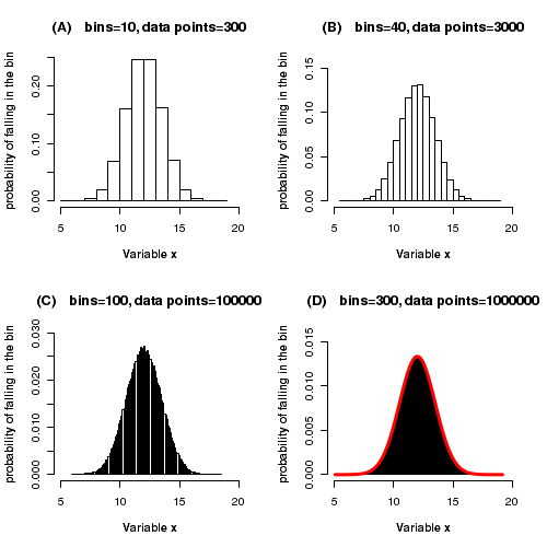
In the four plots given above, we see that as the number of bins increases, the bin width decrease and the probability histogram starts looking like a continuous curve (shown as red line in the fourth plot). We can think other way around. In nature, some populations have continuous distribution. The values of the data points are continuous such that in any given range we can have infinite number of data points. Thus, between 12.4 and 12.5 range, we can have infinite values like 12.45, 12.4532, 12.453219, .... Unless we round them up to finite number of digits, no two numbers from such distributions can be same. Between any two values, there will be infinite number of possible data points. Therefore, we cannot talk of frequency of a particular n that for a continuous distribution. We can only count the number of data points whose values are between two numbers. This means we can plot only a frequency histogram with a bin width for a continuous data. Such a data can only be represented as a continuous distribution, described by a continuous curve when the data size is infinite..
An important difference between continuous and discrete probability distributions of populations
When we plotted the probability distribution of a discrete data, the X-axis represented the discrete value of a variable x, and the Y axis represented the probability of geting a value x in the data . The distribution of a continuous data has a different property.
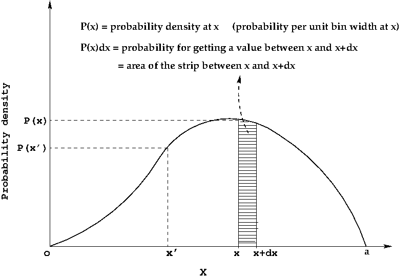
To understand this point, we will draw the probability distribution of a continuous variable x represented by some mathematical function P(x), as shown here:
In a discrete probability distribution, the variable x takes discrete values, and probability of all these discrete values sum to total probability 1.
In a continuous probability distribution, the variable x can take infinite number of values in a given range. Since the probabilities of all these infinite values should sum to one, it is clear that the probability of individual x values should be infinitesmally small. Therefore, in a continuous distribution, we do not consider the probability of observing a given x value. We consider the probability of observing a value within a unit interval around x, called as probability density P(x) .
If P(x) is the probability per unit interval around x (probability density), then P(x)dx gives the probability of observing a value within an interval dx around the value x.
As depicted in the diagram above, P(x)dx is the area of the probability density curve under a strip of width dx around x. This is equal to the probability of sampling a value within width dx around x.
What is the probability of observing an x value between x=1 and x=b?. This is given by the area under the curve between x=a and x=b. This area is obtained by the integral \(\int_{a}^{b} P(x)dx \)
To summarize :
The discrete and continuous probability distributions in nature
The data points from an experiment are assumed to have been randomly sampled from a parent population (simply called "population"). Each one of these populations, whether discrete or continuous, is represented by a probability distribution which has a mathematical expression.
The question is, for a given population we sample, who gives us the mathematical expression of the probability or probability density distribution? Mostly they are derived using the fundamental mathematics that governs the underlying phenomena. We will learn about them in the coming sections.
Some of the important discrete ditributions are:- Binomial distribution
- Poisson distribution
- Hypergeometric distribution
- Geometric distribution
- Negative binomial distributionb
- Gaussian distribution
- Uniform distribution
- Exponential distribution
- Gamma distribution
- Chi-square distribution
- Student's t distribution
- F distribution