CountBio
Mathematical tools for natural sciences
Biostatistics with R
Histograms
A histogram represents the frequency distribution of a data set. A data set is divided into intervals, and the number of data points lying in each interval is plotted against the interval as a rectangular bar.
In R, we can generate histograms using the hist() function. The arguments of this function are almost same as that of plot().
An important parameter of the histogram is the number of intervals (called "bins") into which the data is divided . This number is in turn limited by the number of data points we have. For a given number of data points, if the number of bins are too large, the data will be spread across many bins, thus reducing the number of data points per bin which results in a poor statistics. On the other hand, if the number of bins is too small, the shape of the frequency distribution will be compressed, reducing the resolution. The number of bins have to be optimised for a given number of data points.
The hist() function has a parameter called breaks that takes an integer value to create that many bins in the histogram.
The following script creates a vector of data and plots the histogram using hist() function. We set the number of data bins as 7 through the function parameterbreaks=7. The resulting histogram is shown below the code:
length = c(10.2, 11.9, 11.3, 12.2, 12.7, 12.8, 14.3, 14.5, 14.6, 15.9,
                  14.8, 15.0, 15.5, 13.2, 13.9, 18.5, 18.9, 18.4, 18.9,
                  19.0, 19.5, 16.1, 16.2, 16.5, 16.8, 16.9, 16.7, 17.3,
                  20.2, 20.5, 20.9, 20.8, 20.2, 22.5, 22.7, 22.9)

hist(length, breaks=7, main="Simulated Data")

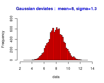
As a second example, we will create 10000 random deviates drawn from a Gaussian distribution of mean 8.0 and standard deviation 1.3. When we plot the histogram of these 10000 random points, we should get back an approximately bell shaped Gaussian curve.
R has a library function called
The R script for creating this histogram is shown below along with the plot. In the plot, we are dividing the data set into 40 equal bins by setting breaks=40.
# Generate 10000 Gaussian deviates with mean=8, and Standard deviation=1.3
data = rnorm(10000, mean=8, sd=1.3)

#plot histogram with 40 bins
hist(data, breaks=40, col="red", xlim=c(2,14), ylim=c(0,800),
              main="Gaussian deviates :  mean=8, sigma=1.3", col.main="blue")
Accessing the results of the histogram
We can also access the data of the histogram through the object returned by the histogram. Try this script:
 Generate Gaussian deviates with mean=5, and SD=3
data <- rnorm(10000, mean=5, sd=3)

#plot histogram with 40 bins and get the returned histogram object.
hdat <- hist(data, breaks=40, col="red", xlim=c(-10,20), ylim=c(0,800),
                      main="Simulated Data", col.main="blue")

# print the contents of hist, which has histogram data
print(hdat)

# we can access (for example) first 10 elements of bin data
print( hdat$breaks[1:10])

# we can access (for example) first 10 elements of counts on bins
print(hdat$counts[1:10])

# First 10 elements of Intensities
print(hdat$intensities[1:10])

## First 10 elements of Kernal Densitieshdat
print(hdat$density[1:10])

# First 10 elements of mid values
print(hdat$mids[1:10])