CountBio

In the previous section we learnt that for n data points randomly drawn from a Normal distribution \(\small{N(\mu,\sigma)}\), the computed sample mean \(\small{\overline{x}}\) also follows a Normal distribution \(\small{N(\mu,\dfrac{\sigma}{\sqrt{n}})}\).

This result is very useful due to the following reason.Since the distribution of \(\small{\overline{x}}\) follows the Normal distribution \(\small{N(\mu,\dfrac{\sigma}{\sqrt{n}})}\), we can do the Z tranformation to get,

\(~~~~~~~~~~~~~~~~~~~~~ \small{Z = \dfrac{\overline{x} - \mu}{\left(\dfrac{\sigma}{\sqrt{n}}\right)} = N(0,1) }\)

Given the values of \(\small{\overline{\mu}, \sigma}\) of the population and sample size \(\small{n}\), we can compute Z value for the sample mean \(\small{\overline{x}}\). Then, using the unit normal table, we can compute the probability of getting a mean value more than the observed \(\small{\overline{x}}\). This gives us a sense of how rare it is to observe this sample mean from \(\small{n}\) random samples.

What happens when the population from which we sample follows a distribution that is not Gaussian. What will be the distribution of sample mean computed using points drawn from non-normal distribution?.

If the distribution of sample mean depends on the population distribution from which data are drawn, we may end up with innumerable number of distributions to compute the significance of observed mean. We are saved from this difficulty by the Central Limit Theorem , the most important theorem of the frequentist method. According to this theorem, the mean sampled from even non-normal distribution follows a Gaussian in the limit of very large sample size!. We will now state and explain the theorem without providing its proof.

The statement of the central limit theorem

If \( \small{\overline{x} }\) is the mean value of a random sample of size n drawn from a distribution of finite mean \( \small{\mu }\) and finite positive variance \( \small{\sigma^2}\), then the distribution of
\(~~~~~~~~~~~~~~~~~\small{Z = \dfrac{\overline{x} - \mu}{\left(\dfrac{\sigma}{\sqrt{n}}\right)} ~~~is~~~N(0,1)}~~in~the~large~limit~~n\rightarrow \infty\)

The central limit theorem states that even if we sample from a non-normal distribution, the computed mean mean using n samples behaves as if it is from a near gaussian distrbution provided the sample size is large!.

This makes our life simple sice we can use the same normal distribution tables, formulas for the estimating the probability of smaple mean \( \small{\overline{x} }\) from the data, even if it is samples from a non Gaussian distribution! So long as the sample size is large, the Gaussian approximation is good enough.

How large the sample size should be for applying the central limit theorem?

In the statement of the central limi theorem, we see that the sample size n tends to infinity. However, in a practical data analysis, the following approximations are kept in mind:

• If the population is exactly Gaussian, then the distribution of the sample mean \( \small{\overline{x} }\) gauranteed to be Gaussian. In this case, the central limit theorem is valid even if the sample size is as small as 3 or 4.


• If the population is nearly gaussian or a distribution that is symmetric about the mean, then the distribution of sample mean \( \small{{x} }\) is nearly Gaussian, and the central limit theorem can be applied with moderate number of sample data points (say, 8 or 10 data points).


• If the population is non-Gaussian, or we do not know anyhing about it, then we may require a large number of sample data points for applying the central limit theorem. One rule of the thumb is, if the data points are more than 30 in number, central limit theorem can approximately applied to any distribution, and this approximation improves more and more as sample size increases further. If, for example, our sample size is more than 60, we can safely apply central limit theorem to data sampled from any distribution.

Demonstration of the Central Limit Theorem with simulated data

We can check whether central limit theorem is really followed by a non Gaussian data set using random deviates in R statistical package. We will choose a uniform density distribution in a range \([a,b]\) defined by,
\( \small{P(x) = \dfrac{1}{b-a} ~~~~~ for~~a \lt x \lt b} \), and \(\small{P(x) = 0 }\) outside the range.

Suppose we let \(\small{a=0, b=10}\). Then we can compute the population mean and variance of this distribution as,
\(\small{\mu = \displaystyle{\int_0^{10}} xP(x) = \displaystyle{\int_0^{10}} x (\dfrac{1}{b-a})dx = \displaystyle{\int_0^{10}} x (\dfrac{1}{10-0})dx = 5 }\)

\(\small{\sigma^2 = \displaystyle{\int_0^{10}} (x-\mu)^2 P(x)dx = \displaystyle{\int_0^{10}} (x-\mu)^2 (\dfrac{1}{10-0} )dx = 3.5714 }\)

Therefore, \(~~~ \small{\sigma = \sqrt{3.5714} = 1.8898 } \)





We will now generate 100000 data points (a very large number) from a uniform distribution in the range [0,10] using the R library function runif(). The frequency histogram of these data points must have uniform distribution.
From this uniform distribution, we randomly sample 10 data points and compute their mean \( \small{\overline{x} }\). We then compute the Z tranformation, \(~~~\small{Z = \dfrac{\overline{x} - 5}{\left(\dfrac{1.8898}{\sqrt{n}}\right)}}\)





We repeat this exercise to draw 100000 random samples of size 10 and compute the Z values for each one of them. The histogram of these Z values, according to Central Limit theorem, must be a unit gaussian!.





See the Figure below:

Freqeucy distribution of sample from Uniform distribution and its Z transformation

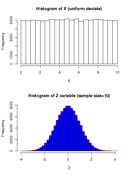
In the above figure, the plot on the top is the frequency distribution of Uniform distribution in the range [0,10]. The blue coloured histogram at the borrom shows the distribution of mean \( \small{\overline{x} }\) of 10 samples randomly drawn from the distribution. The histogram of \(\small{Z = \dfrac{\overline{x} - 5}{\left(\dfrac{1.8898}{\sqrt{n}}\right)} }\) is definitely a Gaussian, as confirmed by the superimposed red color Gaussian curve sitting nicely on the histogram.

This is the power of the Central Limit Theorem : the mean of n samples randomly drawn from a uniform flat distribution follow unit gaussian under Z tranformation. This can also be demonstrated for many skewed distributions that are non-Gaussian.

The R scipt that performs the above mentioned simulation is given below:

####  Applying central limit theorem to Uniform distribution

# For Uniform distribution from min to max,

##  P(x) = 1/(max-min) in the range [min,max]
##       = 0  (outside this range)

## Let min=0, max=10

##  population mean = mu = integral from min to max of ( x * P(x) dx)

##                       = integral from 0 to of(x* (1/(max-min)) dx ) 
##                       = 5

##  population variance = sigmasqure = integral from min to max of ( (x-mu)^2 * P(x) dx )
##                                   = integral from 0 to 10 of ( (x-5)^2 * (1/10) dx )
##                                   = sqrt(25/3) =  2.886                                


####

par(mfrow = c(2,1))

## mean and sd of uniform distribution in [0,10], computed as above.
mu = 5  ## 

sigma = sqrt(25/3)  

## plotting the histogram of uniform deviates between [0,10]
X = runif(100000, min=0, max=10)

hist(X, breaks=30, main="Histogram of X (uniform deviate)" )



## randomly drawing 50 data points from uniform distribution in [0,10]
n = 10

Z = c()

## computing the Z variable vector for 100000 data sets of size 50 each.
for( i in 1:100000) {

 y = runif(n, min=0, max=10)

 z = (mean(y) - mu)/(sigma/sqrt(n))

 Z = c(Z,z)

}

## plotting the histogram of Z variable.
 h = hist(Z, breaks = 30, col="blue", main="Histogram of Z variable (sample size=10)")

## draw a Gaussian curve 
xfit<-seq(min(Z),max(Z),length=60) 
yfit<-dnorm(xfit,mean=mean(Z),sd=sd(Z)) 
yfit <- yfit*diff(h$mids[1:2])*length(Z) 
lines(xfit, yfit, col="red", lwd=1)

Problem solving with Central Limit Theorem