CountBio

According to the Central Limit Theorem, the sample mean \(\small{\overline{x}}\) estimated from n random samples from a distribution will be unit normal under the tranformation,

\(~~~~~~~~~~~~~~~~~\small{Z = \dfrac{\overline{x} - \mu}{\left(\dfrac{\sigma}{\sqrt{n}}\right)} ~~~is~~~N(0,1) }\)

See figure below:

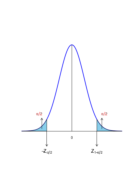
For a given set of values for \( \small{\overline{x}, \mu~and~\sigma}\), let \(\small{\alpha}\) be the probability of getting Z values above and below a threshold.

Let, \(Z_{1-\alpha/2} ~\) be the Z value above which the area under the curve is \(\small{\dfrac{\alpha}{2} }\). This means, \(~\small{P(Z \gt Z_{1-\alpha/2}) = \dfrac{\alpha}{2}}\)

Similarly, \(-Z_{1-\alpha/2} ~\) be the Z value below which the area under the curve is \(\small{\dfrac{\alpha}{2} }\). ie., \(~\small{P(Z \lt -Z_{1-\alpha/2}) = \dfrac{\alpha}{2}}\)

The probability for a Z value in the range \(\small{[-Z_{1-\alpha/2}, Z_{1-\alpha/2}]}\) is \(\small{1-\alpha }\). Therefore, we write this as,

\( ~~~~~~~~\small{P(-Z_{1-\alpha/2} ~\leq ~Z \leq ~Z_{1-\alpha/2}) = 1-\alpha }\)

Substituting for Z the expression of Z tranform, we get

\( ~~~~~~~~\small{P(-Z_{1-\alpha/2} ~\leq ~\dfrac{\overline{x} - \mu}{\left(\dfrac{\sigma}{\sqrt{n}}\right)} \leq ~Z_{1-\alpha/2}) = 1-\alpha }\)

We now consider the following inequality :

\(~~~~~~~~\small{ -Z_{1-\alpha/2} ~\leq ~\dfrac{\overline{x} - \mu}{\left(\dfrac{\sigma}{\sqrt{n}}\right)} \leq ~Z_{1-\alpha/2} }\)

Multiplying throughout by \(\small{\dfrac{\sigma}{\sqrt{n}} }\), we get

\(~~~~~~~~\small{ -Z_{1-\alpha/2}\left(\dfrac{\sigma}{\sqrt{n}}\right) ~\leq ~\overline{x} - \mu \leq ~Z_{1-\alpha/2}\left(\dfrac{\sigma}{\sqrt{n}}\right) }\)

We add \(\small{-\overline{x}}\) throughout to get

\(~~~~~~~~\small{-\overline{x} -Z_{1-\alpha/2}\left(\dfrac{\sigma}{\sqrt{n}}\right) ~\leq ~ -\mu ~ \leq ~-\overline{x} + Z_{1-\alpha/2}\left(\dfrac{\sigma}{\sqrt{n}}\right) }\)

Multiplying throught by -1, we can reverse the inequality to get:

\(~~~~~~~~\small{\overline{x} + Z_{1-\alpha/2}\left(\dfrac{\sigma}{\sqrt{n}}\right) ~\geq ~ \mu ~ \geq ~\overline{x} - Z_{1-\alpha/2}\left(\dfrac{\sigma}{\sqrt{n}}\right) }\)

reading this from left, we get the final result

\(~~~~~~~~\small{\overline{x} - Z_{1-\alpha/2}\left(\dfrac{\sigma}{\sqrt{n}}\right) ~\leq ~ \mu ~ \leq ~\overline{x} + Z_{1-\alpha/2}\left(\dfrac{\sigma}{\sqrt{n}}\right) }\)

With the above inequality, we can make this final statement:

The above result is a remarkable one. It says the following:

Once the sample set X is measured and sample mean \(\small{\overline{x}}\) is computed, we can construct an interval \(\small{\overline{x} \pm Z_{1-\alpha/2}\left(\dfrac{\sigma}{\sqrt{n}}\right)}\) around this mean.

We can say with \(\small{(1-\alpha)\times 100\% }\) confidance that the unknown population mean \(\small{\mu }\) is in this interval, provided we know the population standard deviation \(\small{\sigma }\).

The interval
\(\small{\overline{x} \pm Z_{1-\alpha/2}\left(\dfrac{\sigma}{\sqrt{n}}\right)}\)




is called the Confidence interval on the population mean

For example, for a given data set, let us fix \(\small{\alpha = 0.05}\). Then \(~~\small{\dfrac{\alpha}{2} = 0.025 }\) and \(~~\small{1 - \dfrac{\alpha}{2} = 0.975 }\). We thus have,

\(\small{\overline{x} \pm Z_{0.975} \dfrac{\sigma}{\sqrt{n}}}\) as the \(\small{95\% }\) confidence interval around the estimated mean \(\small{\overline{x} }\). We have to get \(\small{Z_{0.975} }\) from Gaussian table.

Understanding the confidence interval on population mean

Suppose we randomly draw \(\small{n}\) data points from a distribution with a given \(\small{\mu}\) and \(\small{\sigma}\). We compute, say, a \(\small{95\%}\) condifence interval on population mean for this sample data. The population mean \(\small{\mu}\) may or may not be within this interval. Now we repeat this whole exercise m times (we call it "m experiments") where m is large. Everytime we pick n random samples, get the sample mean, compute the \(\small{95\%}\) confidence interval and check whether the population mean \(\small{\mu}\) is inside the interval . Note that every time, the population mean will be different, and hence the confidence interval. We expect that out of m such experiments, \(95\%\) of the cases will have the population mean within the confidence interval and \(5\%\) of them will have population mean outside the interval.

The confidence interval does not say that \(\small{\mu}\) assumes a value within the interval with a probability 0.95. It does not say anything about the value of \(\small{\mu}\).

Two sided and One sided confidence intervals

The confidence interval \(\small{\overline{x} \pm Z_{1-\alpha/2}\left(\dfrac{\sigma}{\sqrt{n}}\right)}\) gives the \(\small{(1-\alpha)100\%}\) confidence with which we say that the population mean is in the given interval.

This expression gives a two sided confidence interval, since the given \(\small{\alpha}\) is split between the lower and upper bounds of the interval.

Sometimes, we want to estimate only the lower or upper bound within which \(\small{\mu}\) can be located with \(\small{(1-\alpha)100\%}\) confidence. In this case, the entire probability \(\small{\alpha}\) is assigned to one side.

An \(\small{(1-\alpha)100\%}\) upper one sided confidence interval on \(\small{\mu}\) is written as, \(\small{\overline{x} + Z_{1-\alpha}\left(\dfrac{\sigma}{\sqrt{n}}\right)}\)

Similarly, we can write a \(\small{(1-\alpha)100\%}\) lower one sided confidence interval on \(\small{\mu}\) as, \(\small{\overline{x} - Z_{1-\alpha}\left(\dfrac{\sigma}{\sqrt{n}}\right)}\)

Thus, in the case of one sided interval, we compute \(\small{Z_{1-\alpha}}\) instead of \(\small{Z_{1-\alpha/2}}\).