CountBio
Mathematical tools for natural sciences
Basic Statistics with R
The t distribution
In the previous two sections we learnt that even if a distribution does not follow Gaussian exactly, we can use the central limit theorem to construct a confidence interval on population mean if the number of data points \(\small{n }\) is large. For this we assumed that the Z statistic defined by \( \small{Z = \dfrac{\overline{x} - \mu}{\left(\dfrac{\sigma}{\sqrt{n}}\right)} }\) is unit normal. We definitely need the value of \(\small{\sigma}\) for contructing the confidence interval on population mean.
In real life situations, we generally make \(\small{n}\) repeated observations on a variable \(\small{x}\) to get \(\small{n}\) data points. We may not get any information on the standard deviation \(\small{\sigma}\) or, for that matter, even on the mean \(\small{\mu}\) of the population. What we can do is to compute the mean \(\small{\overline{x}}\) and standard deviation \(s\) of the sample.
The general belief is that if the data points are large enough (say, more than 30 or 40), we can approximate the computed sample standard deviation \(s\) to be very closely equal to the population standard deviation \(\small{\sigma}\) and then compute the confidence interval.
To what extent \(s\) gets closer to \(\small{\sigma}\) as the sample size increases?
We will do the following simulation in R to answer this question. We consider a Gaussian distribution with a mean value of \(\small{\mu=15}\) and a standard deviation \(\small{\sigma = 3 }\). In R, we can use the function

From the above figure, we learn that as the sample size n increases, the estimated standard deviation \(\sigma\) gets closer and closer to the population standard deviation of \(\sigma=3\), as expected. However, even when the sample size is as large as \(\small{n=60}\), considerable fraction of experiments will have their estimated sample standard deviation considerably different from the population standard deviation of 3. The situation imrpoves to few percent difference only when the sample sizes reach as high as 100.
Therefore, for small sample sizes, we definitely cannot use the computed \(s\) instad of unknown \(\small{\sigma}\) in the above mentioned formulas for applying the central limit theorem. What do we do?
Student's t distribution
This problem of using the sample standard deviation \(s\) instead of \(\small{\sigma}\) was addressed by the English Statistician William Sealy Gosset in the journal Biometrica in 1908 under the pseudonyme "student". See here for the very interesting story behind the discovery of t distribution by Gosset when he was working for a Brewery and why he had to publish it with a pseudonyme "student"!
According to this analysis, when \(s\) replaces \(\small{\sigma}\), the statistic defined by
\(\small{\dfrac{\overline{x} - \mu}{\left(\dfrac{s}{\sqrt{n}}\right)} }\) does not follow a unit normal distribution. Instead, this quantity follows a distribution called t distribution .
For a sample of size \(\small{n}\), this t statistic is written as,
When to use the t distribution
The strict requirement for using the t distribution is that the sample must be drawn from a Gaussian distribution. However, it can be approximately used if the parent distribution is near gaussian (for example, at least an inverted bowel shaped curve if not a nice bell curve). It should not be used for data sampled from any arbitrary shaped non-gaussian parent distributions.
Properties of the t distribution
-
The probability density of a t distribution for a sample of size \(\small{n}\) is defined as, \( \small{P(t,\nu) = \dfrac{\Gamma \left(\dfrac{\nu + 1}{2}\right)}{\sqrt{n\pi}~ \Gamma \left(\dfrac{\nu}{2}\right)} \left(1 + \dfrac{t^2}{\nu}\right)^{-\dfrac{(\nu + 1)}{2} } }\) where \(~~\small{\nu = n-1}~~\)is the degrees of freedom, and \(\small{\Gamma(x)}~~\)is a Gamma function defined by, \(~~\Gamma(x) = \int\limits_0^\infty y^{x-1}e^{-y} dy \) One need not get intimidated by the above formula. Given a sample size \(\small{n}\) and a value of \(\small{t}\) statistics, we can compute probability density as well as area under curve from t using tables and R funcitons, as described in the coming section.
-
Similar to Gaussian distribution, the t distribution has a mean of 0 and is symmetrical about the mean. The variance of the t distribution is greater than 1 for normal sample sizes, and the variance approaches 1 for larger sample sizes. For \(\small{n \gt 3}\), the variance of the t distribution is \(\small{\dfrac{(n-1)}{(n-3)} }\).
-
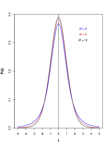
The t distribution is actually a family of distributions, each defined by a value of degree of freedom\(~~\small{n-1}\). Thus, for a given number of samples \(\small{n}\), we should refer to the corresponding distribution \(\small{t(n-1) }\) for computing the probability of getting statistic \(\small{t}\)more than or less than a threshold value. Figure below shows the graphs of t distributions for different degress of freedom \(\small{df = n-1 }\):
-
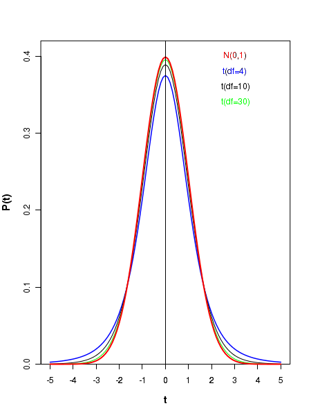
Compared to Gaussian distribution, the t distribution has lesser peak and more slowly falling tail. Hoewever, as the number of degrees of freedom \(\small{df = n-1 }\) increases, the t distribution shape aprroaches that of Gaussian. This is illustrated by a set the comparative curves below. Notice that when \(\small{df=30}\), the T distribution represented by green curve almost sits on the unit normal curve drawn in red color . Theoretically, the t distribution approaches normal distribution as \(\small{n-1 }\) tends to infinity. But for all practical purposes, when \(\small{df \gt 30}\), it approximately looks like a Gaussian.
Computation of probabilities from t distribution
Similar to what we did with the Gaussian distribution, we can compute the probability of getting more than or less than certain value of t statistic. The probability can be one sided or two sided. See the two figures below:
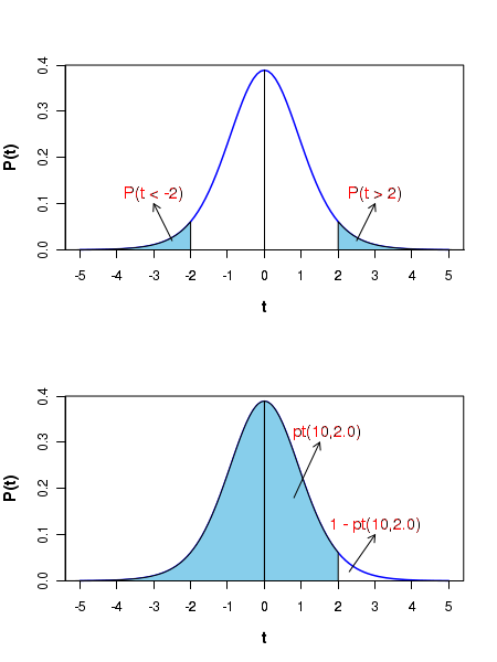
In the above figure, the plot at the top shows the two shaded areas which represent the probabilities above and below particular \(\small{t}\) values. Generally, for various degrees of freedom, the \(\small{t}\) values for which the area under the \(\small{t}\) distribution is \(\small{\alpha}\) is tabulated for selected values of, for example, \(\small{\alpha = 0.001, 0.005, 0.01, 0.05, 0.1}\) etc. This table can be found in the web sites of various academic institutions. One such t-distribution table can be accessed from here. In this table, the \(\small{t}\) values corresponding to \(\small{\alpha = 0.1, 0.05, 0.025, 0.01, 0.005}\) are tabulated for each degrees of freedom from 1 to 30. In this table, for example, corresponding to a degrees of freedom \(\small{df=n-1=10}\), the t-value corresponding to a one tailed probability of 0.025 is 2.228. We write this as, \(~~~~~~~~~~~~~\small{t_{\alpha}(n-1) = t_{0.025}(10) = 2.228} \) This means that for the t-distibution with 10 degrees of freedom, the area under the curve from \(t = 2.228\) to \( t = \infty \) is 0.025. For the same distribution, the area under the curve from \( t = -\infty \) to \(t = -2.228\) is 0.025, since the curve is symmetric about t=0. R provides a function \(~~\small{pt(n-1, t)}\) which returns the area under the t diatribution from \(\small{t = -\infty~to~t}\) for a given degrees of freedom \(\small{df=n-1}\).
Confidence intervals using t distribution
For a data sampled from a distribution of population mean \(\small{\mu }\) and standard deviation
\(\small{\sigma}\), we derived in the previous chapter an expression for the \(\small{(1-\alpha)100\% }\)
two sided confidence interval around population mean as,
\(~~~~~~~~~~~\small{\overline{x} \pm Z_{1 - \alpha/2}\left(\dfrac{\sigma}{\sqrt{n}}\right)}\)
The same concept can be just extended to the t-distribution. When we sample from a normal distribution whose standard deviation is unknown, we can write an expression for a two sided, \(\small{(1-\alpha)100\% }\) confidence interval for population mean as,
In a health survey, 20 random samples of 22 year old Indian women were chosen and their weight was mwasured. The data is presented here: \(\small{X = \{58.5, 64.1, 61.6, 62.2, 62.7, 58.2, 50.4, 55.3, 56.7, 56.8, \\~~~~~~~~ 49.2, 50.3, 54.9, 46.7, 61.3, 55.0, 52.8,5.6, 62.3, 43.4\} }\) Construct a 95 percent confidence interval for this data. Since the individual's height can be more or less than the mean value, we construct a 2 sided confidence interval. From the data, we estimate \(~~~~\small{\overline{x} = 55.9}~~~\) and \(~~~s = 5.7 \). We have \(~~\small{1 - \alpha=0.95 }\). Hence, \(~~~\small{\alpha = 0.05, \dfrac{\alpha}{2} = 0.025}\). The degrees of freedom \(\small{df = n-1 = 20-1 = 19. }\) From the t-distribution table, we note that \(~~~\small{t_{\alpha = 0.025}(19) = 2.093 }\). Therefore, the two sided \(\small{95\% }\) confidence interval can be written as, \(\small{55.9 \pm 2.093 \times \dfrac{5.7}{\sqrt{20}} = (53.23, 58.56) }\)
Now we will learn to use the R library functions for the t distribution.
R scripts
Let t = t distribution variblen = sample sizedf = n-1 = degrees of freedom Then,dt(t, df) -----> returns the probability density at t on a t distribution curve.rt(m, df) -----> returns m random deviates from t distribution with df degress of freedom.qt(p, df) -----> returns the t value corresponding to a cumulative probability p on a t distribtuion with df degrees of freedom.pt(t, df) -----> returns the cumulative probability p from minus infinity to t on a t distribution with df degrees of freedom.
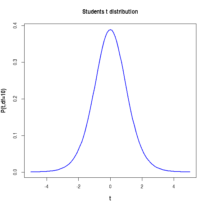
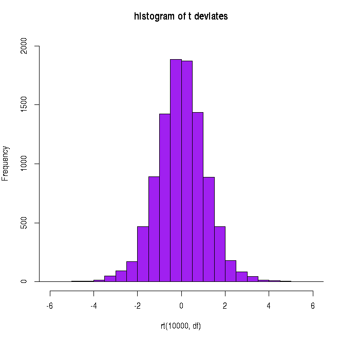
##### Using R library functions for the t distribution

#### probability density function
n = 10
df = n-1
t = 2.5

t_density = dt(t,df)
t_density = round(t_density, digits=2)
print(paste("probability density for t = ", t, " and degree of freedom = ", df, " is ",
               t_density))

### Generating the curve of t distribution probability density

x = seq(-5,5,0.1)

df = 10

string = "P(t,df=10)"

curve(dt(x, df), xlim=c(-5,5), xlab="t", ylab=string, lwd=1.5, cex.lab=1.2, col="blue",
                main="Students t distribution", font.lab=2)


#### Generating cumulative probability (p-value) above upto a t value in a t distribution

#######  pt(t,df) generates cumulative probability from minus infinity to t
#######  when t is positive, probability above t is 1-pt(t)
#######  when t is negative, probability below -t is pt(t)

df=10

t = 2.6
pvalue = pt(t,df)
pvalue = round(pvalue,3)
print(paste("cumulative probability from t = minus infinity to ", t, "is ", pvalue))

t = -2.6
pvalue = pt(t,df)
pvalue = round(pvalue,3)
print(paste("cumulative probability from t = minus infinity to ", t, "is ", pvalue))


#### Generating t value for a cumulative probability p
###  The function qt(p,df) returns t value at which cumulative probability is p.

p = 0.95  ## cumulative probabilitu from minus infinity to t.
t = qt(p,df)
t = round(t, digits=3)
print(paste("t value for a cumulative probability p = ", p, "is ", t))


#### Generating random deviates from a t distribution
### rt(m,df) returns a vector of m random deviates from a t of given df

ndev = rt(4, df)
ndev = round(ndev,digits=3)
print("Four random deviates from t distribution with 10 degrees of freedom : ")
print(ndev)

X11()

## plotting the histogram of 10000 random deviates from unit Gaussian:
hist(rt(10000, df), breaks=40, xlim=c(-6,6) , ylim = c(0, 2000), col="purple",
                main="histogram of t deviates")
Executing the above script in R prints the following results and figures of probability distribution on the screen:
[1] "probability density for t =  2.5  and degree of freedom =  9  is  0.03"
[1] "cumulative probability from t = minus infinity to  2.6 is  0.987"
[1] "cumulative probability from t = minus infinity to  -2.6 is  0.013"
[1] "t value for a cumulative probability p =  0.95 is  1.812"
[1] "Four random deviates from t distribution with 10 degrees of freedom : "
[1]  1.225  0.361  0.214 -1.774