CountBio
Mathematical tools for natural sciences
Basic Statistics with R
Gaussian distribution
The Gaussian distribution (also called "Normal distribution") is the most important continuous distribution in statistics. Repeated measurements of many quantities in nature follow close approximation to Gaussian distribution. Some examples : Hieght and weight of the people, blood sugar, blood pressure, marks in exams, errors on measured quantities etc.
To demonstrate this, we plot the histograms of a real data set that contains heights and weights of 1035 major league basketball players in United States. Data source : from SOCR site http://wiki.stat.ucla.edu/socr/index.php/SOCR_Data_MLB_HeightsWeights

The above two distributions are in the form of a "bell shaped curve". We also notice that the histograms approximately peak at their mean values. Thus, in the case of height, the curve peaks at the mean height of 187.2 cm and the histogram of weight peaks at its mean value of 91.5 Kg.
This bell shaped distribution is universally exhibited by the repeated measurements of many quantities in nature. During 18th and 19th centuries, mathematicians in Europe provided the mathematical formula for this bell shaped probability density distribution. Prominant among them was Gauss, who derived the theoretical probability distribution for this bell shaped curve. This distribution was later referred to as "Gaussian distribution". It is widely known as "Normal distribution". A brief historical note on this distribution is given at the later section.
Gaussian probability density function
The normal (Gaussian) density distribution of a variable with population mean \(\small{\mu}\) and standard deviation \(\small{\sigma}\) is given by,
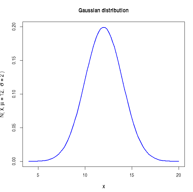
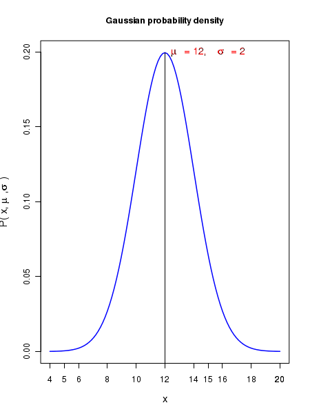
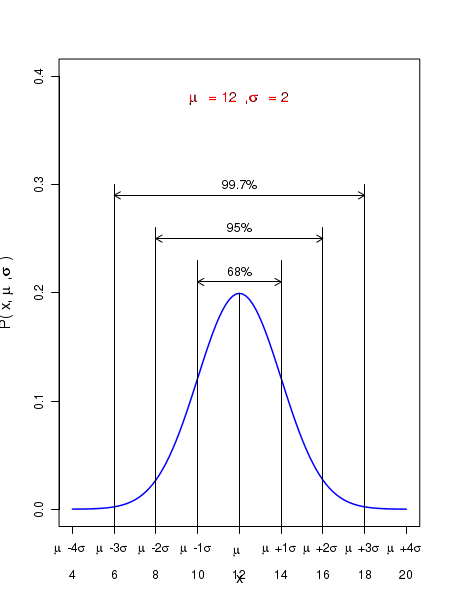
The plot of the above Gaussian density function is shown below for specific values of mean \(\small{ \mu = 12}\) and standard deviation \(\small{\sigma = 2}\):
The Gaussian probability density distribution has the following properties:
- The Gaussian density function represents a continuous distribution defined by two variables, the arithmetic mean \(\small{\mu }\) and the standard deviation \(\small{\sigma}\). Thus \(\small{\mu }\) represents the central tendency and \(\small{\sigma}\) is a measure of spread in the distribution about the mean value.
- The distribution is a bell shaped curve symmetric around the mean value \(\small{\mu }\). Thus for the normal distribution, the mean, median and mode are same.
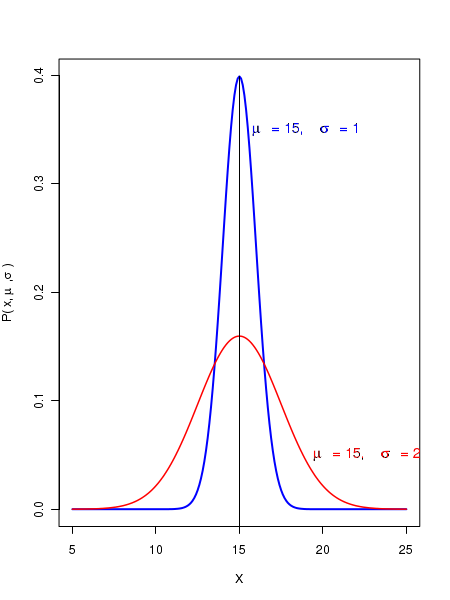
- The parameters \(\small{\mu }\) and \(\small{\sigma }\) are independent of each other. Two distributions can have same mean but different spreads due to difference in their standard deviations. This is shown in the figure below:
-
Since Normal distribution is continuous, P(x) represents the probability of observing a value in a unit interval around x. This is probability density. In order to get the probability of observing a value in an interval \(\small{[a,b]}\), we have to integrate the density function \(\small{ P(x) }~\)from \(~\small{x=a}\) to \(\small{x=b}\): \(\small{P(a \lt x \lt b ) = \displaystyle{\int_a^b} P(x)dx = \displaystyle{\int_a^b} \dfrac{1}{\sigma \sqrt{2\pi}} {\Large e}^{-\dfrac{1}{2}\left(\dfrac{x-\mu}{\sigma}\right)^2} dx}\) $~~~~~~~~~~~~~~~~~~~~~~~~~~~~~~~~~~~~~~~~~~~$= Area under the curve P(x) from x=a to b
-
The total area under the Gaussian curve in the range \(\small{[-\infty, \infty]}\) is unity. The function is defined in such a way that
\(\small{\displaystyle{\int_{-\infty}^\infty} P(x)dx = \displaystyle{\int_{-\infty}^\infty} \dfrac{1}{\sigma \sqrt{2\pi}} {\Large e}^{-\dfrac{1}{2}\left(\dfrac{x-\mu}{\sigma}\right)^2} dx = 1}~~~~\)
We say that the curve is "normalized" in the range of \(\small{x}\)). -
Though the range of the variable \(\small{x}\) extends to infinity on both sides, the probability density \(\small{P(x)}\) falls as a function of \(\small{x}\) such that very few events are left after a distance of 3 standard deviations away from the mean value. It helps to remember the following three numbers: About \(\small{68\%}\) of the data points are within \(\pm 1\) standard deviation from mean. About \(\small{95\%}\) of the data points are within \(\pm 2\) standard deviation from mean. About \(\small{99.7\%}\) of the data points are within \(\pm 3\) standard deviation from mean. In the probability density curve, the same statements translate into \(~~~~~P(\overline{x} \pm 1\sigma)~\approx 0.68 \) \(~~~~~P(\overline{x} \pm 2\sigma)~\approx 0.95 \) \(~~~~~P(\overline{x} \pm 3\sigma)~\approx 0.997 \) These ranges are illustrated in the figure below:
The Normal distribution has the following important convolution properties: 1. The sum of two Gaussian variables is also a Gaussian. If variable \( X_1 \sim N(\mu_1, \sigma_1^2)\) and \(X_2 \sim N(\mu_2, \sigma_2^2)\), then \(X_1 + X_2 \sim N(\mu_1 + \mu_2, \sigma_1^2 + \sigma_2^2) \). 2. We can scale a normally distributed variable: If \( X \sim N(\mu, \sigma^2)\), then the scaled variable \(~~~ kX \sim N(k\mu, k^2\sigma^2)\)
The unit normal distribution
The Gaussian function \(\small{P(x) = \dfrac{1}{\sigma \sqrt{2\pi}} {\Large e}^{-\dfrac{1}{2}\left(\dfrac{x-\mu}{\sigma}\right)^2} }\) can be analytically integrated in the interval \(\small{[-\infty,\infty]}\). However, the analytical integration of this function does not exist in a finite interval \(\small{[a,b]}\). Numerical methods must be employed to get the area under the Gaussian curve in a finite interval.
This process can be made simple by applying a simple transformation to the Gaussian probability density formua:
Substituting \(\small{Z = \dfrac{x-\mu}{\sigma}}\) in the Gaussian function \(\small{P(x) = \dfrac{1}{\sigma \sqrt{2\pi}} {\Large e}^{-\dfrac{1}{2}\left(\dfrac{x-\mu}{\sigma}\right)^2} }\), we get
\(\small{\displaystyle{\int P(x)dx} = \displaystyle{\int\dfrac{1}{\sigma \sqrt{2\pi}} {\Large e}^{-\dfrac{1}{2}\left(\dfrac{x-\mu}{\sigma}\right)^2} dx = \displaystyle{\int\dfrac{1}{\sqrt{2\pi}} {\large e}^{-\frac{Z^2}{2}} dz }}}\)
The function inside the last integral is called the unit normal distribution or unit Gaussian . It is defined as,
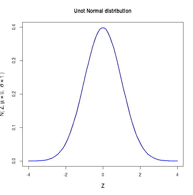
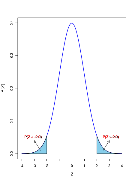
The unit normal distribution is plotted below:
The unit normal distribution has the following properties:
- The distribution has zero mean and variance equal to 1.
- The shape is exactly same as that of Gaussian, with mean,median and mode at the peak of the distribution.
-
Any Gaussian distribution with population mean \(\small{\mu}\) and population standard deviation \(\small{\sigma}\) will become unit normal distribution under the tranformation \(\small{Z = \dfrac{x-\mu}{\sigma} }\). We therefore have,
\(\small{ P(x_1 \lt x \lt x_2) = \displaystyle{\int_{z_1}^{z_2}\dfrac{1}{\sqrt{2\pi}} {\large e}^{-\frac{Z^2}{2}} dz } } ~~~~~~~~~~~\) where \(~~~\small{z_1 = \dfrac{x_1-\mu}{\sigma} }~~~\)and \(~~~\small{z_2 = \dfrac{x_2-\mu}{\sigma} }~~~\)
The Unit Gaussian distribution cannot be integrated over finite limits. However, numerical integration of this integral is performed from 0 to various upper limits, and the results are available as tables. Using these Gaussian integral tables, we can get the probability \(\small{P(z_1 \lt Z \lt z_2 ) }\) for the cooresponding range \(\small{(x_1,x_2)}\).
Almost all text books on statistics have the unit Gaussian table at the Appendix section. Many institutions and individuals have created and kept the tables in the web. For example, a table containing the integration of unit normal distribution from \(\small{-\infty}\) to various values of \(\small{Z}\) from -3.4 to +3.4 can be accessed from here.
-
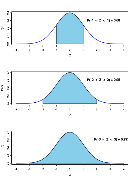
Similar to the Gaussian, the unit normal distribution has the following areas under one, two and three standard deviation ranges:
The area under the curve between Z = -1 to Z = 1 is approximately 0.68.
ie, \(P(-1 \lt Z \lt +1 \approx 0.68 ) \)
The area under the curve between Z = -2 to Z = 2 is approximately 0.95.
ie, \(P(-2 \lt Z \lt +2 \approx 0.95 ) \)
The area under the curve between Z = -3 to Z = 3 is approximately 0.997
ie, \(P(-3 \lt Z \lt +3 \approx 0.997 ) \)
This is highlighted by the shaded areas in the following figure:
Unit Gaussian curve with experimental data
In order to test the concept of unit normal curve with a real data set, we consider the SOCR simulated data on the height measurement of 25000 school students. This data can be accessed in the following link: http://socr.ucla.edu/docs/resources/SOCR_Data/SOCR_Data_Dinov_020108_HeightsWeights.html
We first plot the histogram of the data. Since the number of data points are as high as 25000, we safely assume that the data mean and standard deviation are approximately same as their population values. treating them as population values, we construct the histogram of \(\small{Z = \dfrac{x-\mu}{\sigma} }\) for all height values. We then superimpose the Unit Normal curve \(\small{y = \large{e}^{-(\frac{Z^2}{2})}}\) on the histogram. See the figure below:
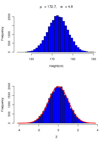
In the above figure, the top curve is the histogram of the height of 25000 students. This data has a mean of 172.7 and standard deviation of 4.8. In the bottom curve, the histogram of the corresponding Z variable given by \(\small{Z = \dfrac{x-172.7}{4.8} }\) is plotted. The red line on the bottom hostogram is the plot of the function \(\small{Frequency = 25000 \times \large{e}^{-(\frac{Z^2}{2})}}\) in the Z range of [-4,4] superimposed on the histogram.
We notice that the match between the histogram and the theoretical Gaussian curve is quiet good, indicating that the data is well represented by the Gaussian distribution
A brief history of the Gaussian distribution
The binomial distribution for observing \(\small k \) success in \(\small n \) Bernoulli trials, with probability of success \(\small p \) for a single trial is given by, \(~~~~~~~~~~~~\small {P(k,n,p) = {_n}C_k p^k q^{n-k}} ~~~\) where \( q = 1-p\) In the earlier 18th century, attempts were made to sum a large number of terms in the binomial distribution. Mathematicians were interested in computing binomial probability for a \(\small{k}\) value in a large range \( \small{k = (k_1,k_2) }\). Computing large sums like the one below were computational challenge:, \(~~~~~~~~~~~~\small{P(k_1 \lt k \lt k_2) = \sum\limits_{k=k_1}^{k_2} {_n}C_k p^k q^{n-k} } \) de Moivre (1733) showed that this large summation can be approximated by the integration of a continuous function for a special case of \(\small{p=\dfrac{1}{2}}\). In 1783, Laplace showed this continuous approximation to be true for \( \small{0 \lt p \lt 1 }\). The integral approximation form to the binomial sum can thus written as de Moivre-Laplace limit theorem: $$\small{P(k_1 \lt k \lt k_2) = \sum\limits_{k=k_1}^{k_2} {_n}C_k p^k q^{n-k} \approx \dfrac{1}{\sqrt{2\pi}} \int_{x_1}^{x_2} e^{-x^2} dx ~~~~~where~~~x_1 = \dfrac{k_1-np}{\sqrt{npq}},~~~x_2 = \dfrac{k_2-np}{\sqrt{npq}} } $$
This integral could be evaluated by numerical methods and tabulated. It is an easy way of estimating cumulative probabilities for binomial distribution.In 1809, Carl Friedrich Gauss, the great German mathematician, developed the formula for the normal distribution from basic assumptions and used it to fit astronomical data. The normal distrbution was also names as the "Gaussian distribution".
Quetelet(1796-1894), the inventor of Body Mass Index, was the first mathematician to apply normal distribution to describe human physical characteristics like hight, weight etc.
The distribution of weight (in Kg) of a certain population of male students is found to follow a Gaussian with a population mean of 57.6 Kg and a standard deviation of 5.2 Kg. Compute the probability that a randomly selected person from the population (a) weighs more than 70 Kg (b) weighs less than 43 Kg (c) weighs in range of 65 to 75 Kg. Given that the weight in Kilograms follows a Gaussian with \(\small{\mu = 57.6 }\) and \(\small{\sigma = 5.2 }\). (a) We compute the probability that a randomly selected person weights more than 70Kg as follows: For \(\small{x=70}\), we have the Z value \(~~\small{Z = \dfrac{(x-\mu)}{\sigma} = \dfrac{70-57.6}{5.2} = 2.4 } \) The probability of weight greater than 70 is same as the probability of \(\small{Z \gt 2.4}\) in the unit normal distribution. From the unit Gaussian table, we read the unit normal probability of getting a value from \(\small{-\infty~to~2.4}\) to be 0.9918. Therefore, \(\small{ P(Z \gt 2.4)~=~1 - P(-\infty \gt Z \gt 2.4)~=~1 - 0.9918 ~=~0.0082}\) (b) In the same way, the probability that a randomly selected person from this population weights less than 43 Kg can be computed as, \(~~\small{Z = \dfrac{(x-\mu)}{\sigma} = \dfrac{43-57.6}{5.2} = -2.8 } \) Then, from the table, \(\small{~~~~P(Z \lt -2.8)~=~P(-\infty \lt Z \lt -2.8)~=~0.00249}\) (c) In order to compute the probability of having a value within 65 to 70 Kg, we should compute the corresponding Z values: \(~~\small{Z_1 = \dfrac{(x_1-\mu)}{\sigma} = \dfrac{65-57.6}{5.2} = 1.42 } \) \(~~\small{Z_2 = \dfrac{(x_1-\mu)}{\sigma} = \dfrac{75-57.6}{5.2} = 3.34 } \) \(\small{P(65 \lt x \lt 75) = P(1.42 \lt Z \lt 3.34) = P(-\infty \lt Z \lt 3.34) - P(-\infty \lt Z \lt 1.42) }\) \(\small{~~~~~~~~~~~~~~~~~~~~~~~~~~~~~~~~~~~~~~~~~~~~~~~~~~~~~~~= 0.9996 - 0.9222}\) \(\small{~~~~~~~~~~~~~~~~~~~~~~~~~~~~~~~~~~~~~~~~~~~~~~~~~~~~~~~ = 0.077 }\)
Gaussian approximation to discrete distribution
A distribution followed by a discrete random variable \(\small{x}\) can be approximated by a Gaussian distribution using the Z transformation \(~~\small{Z = \dfrac{(x-\mu)}{\sigma} }\), where \(\small{\mu}\) and \(\small{\sigma}\) are the population mean and standard deviation of discrete distributions.
For example, if the sampling distribution is binomial \(\small{b(n,p)}\), we have \(\small{\mu = np}\) and \(\small{\sigma = np(1-p)}\). Similarly, if the sampling distribution is Poisson \(\small{P(\mu) }\), \(\small{\mu = \mu}\) and \(\small{\sigma = \sqrt{\mu}}\)
The correction for continuityWhile approximating a discrete distribution to Gaussian, we should apply a correction for continuity . Since the variable \(\small{x}\) is discrete, we should write, \(~~~~\small{Z = \dfrac{(x+0.5) - \mu}{\sigma}~~~~~~~~for~~x \lt \mu }\) \(~~~~\small{Z = \dfrac{(x-0.5) - \mu}{\sigma}~~~~~~~~for~~x \gt \mu }\) where \(\small{\mu}\) and \(\small{\sigma}\) are the population mean and standard devistion of discrete distribution.
We will now learn to compute Gaussian probability distributions in R.
R scripts
For the Gaussian distribution, the following four functions are provided in R for computing various quantities related to the distribution.
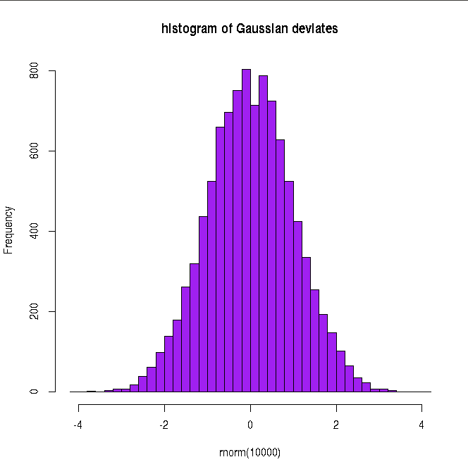
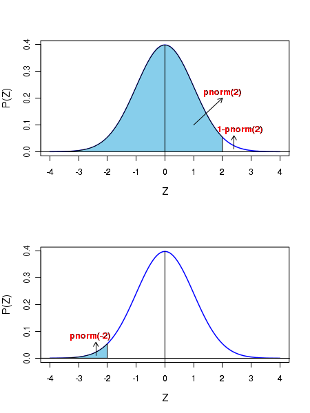
Let Z = Gaussian Z variblemean = the mean value of Gaussian distributionsd = standard deviation of the Gaussian distribution Then,dnorm(Z) ---------------> returns the Gaussian density at Z on a unit normal curve.rnorm(n) ---------------> returns n random deviated unit normal curve.qnorm(p) ---------------> returns the Z value corresponding to a cumulative probability p.pnorm(Z) ---------------> returns the cumulative probability p from minus infinity to Z. See the two plots in the figure below to compute the shaded areas for positive and negative Z using pnorm(Z):
##### Using R library functions for the Gaussian distribution

mean = 12     ## mean of the Gaussian
standev = 2.0 ## means of the standard deviation
x = 14.0    ## Gaussian variable value


### Probability density function

### dnorm(x,mu,sigma)  returns Gaussian probability density for given x,mu,sigma
gauss_density = dnorm(x,mean,standev)
gauss_density = round(gauss_density, digits=3)
print(paste("Gaussian probability for (",x,",",mean,",",standev,") = ", gauss_density) )

### dnorm(Z) returns a probability density for a given Z in unit Gaussian.
Z = 2.0
unit_norm = dnorm(Z)
unit_norm = round(unit_norm,3)
print(paste("Unit Gaussian probability for  Z = ",Z," is ",unit_norm ) )

###  Plotting the Gaussian curve in the x range of (mu - 4*sigma, mu + 4*sigma)
 mean = 12
 standev = 2
 x = seq(mean - 4*standev, mean + 4*standev, 100)
 string =  substitute( paste("N( x, ", mu, " = 12,  ", sigma, " = 2 " , ")"  ))
 curve(dnorm(x, mean, standev), xlim=c(mean - 4*standev, mean +  4*standev),
              ylab=string, lwd=1.5, cex.lab=1.2, col="blue", main="Gaussian distribution")

X11()

## Plotting unit Gaussian curve
 mean = 0
 standev = 1
 x = seq(mean - 4*standev, mean + 4*standev, 100)
 string =  substitute( paste("N( Z, ", mu, " = 0,  ", sigma, " = 1 " , ")"  ))
 curve(dnorm(x, mean, standev), xlim=c(mean - 4*standev, mean +  4*standev),
            xlab="Z", ylab=string, lwd=1.5, cex.lab=1.2, col="blue", main="Unot Normal distribution")

X11()

#### Generating cumulative probability (p-value) above upto a Z value in a unit Gaussian

#######  pnorm(Z) generates cumulative probability from minus infinity to Z
#######  when Z is positive, probability above Z is 1-pnorm(Z)
#######  when Z is negative, probability below Z is pnorm(Z)

Z = 2.6
pvalue = pnorm(Z)
pvalue = round(pvalue,3)
print(paste("cumulative probability from Z = minus infinity to ", Z, "is ", pvalue))

Z = -2.6
pvalue = pnorm(Z)
pvalue = round(pvalue,3)
print(paste("cumulative probability from Z = minus infinity to ", Z, "is ", pvalue))


#### Generating Z value for a cumulative probability p
###  The function qnorm(p) returns Z value at which cumulative probability is p.

p = 0.95  ## cumulative probabilitu from minus infinity to Z.
Z = qnorm(p)
Z = round(Z, digits=3)
print(paste("Z value for a cumulative probability p = ", p, "is ", Z))


#### Generating random deviates from a Gaussian
### rnorm(n,mean, standev) returns a vector of n random deviates from a
####     Gausian N(mean, standev).
### rnorm(n) returns a vector of n random deviates from a Gaussian  N(0,1)

ndev = rnorm(4, mean=15, sd=3)
ndev = round(ndev,digits=3)
print("Four Gaussian deviates from N(15,3) : ")
print(ndev)

## plotting the histogram of 10000 random deviates from unit Gaussian:
hist(rnorm(10000), breaks=30, col="purple", main="histogram of Gaussian deviates")
Executing the above script in R prints the following results and figures of probability distribution on the screen:
[1] "Gaussian probability for ( 14 , 12 , 2 ) =  0.121"
[1] "Unit Gaussian probability for  Z =  2  is  0.054"
[1] "cumulative probability from Z = minus infinity to  2.6 is  0.995"
[1] "cumulative probability from Z = minus infinity to  -2.6 is  0.005"
[1] "Z value for a cumulative probability p =  0.95 is  1.645"
[1] "Four Gaussian deviates from N(15,3) : "
[1] 19.912 14.529 18.494 10.914