CountBio
Mathematical tools for natural sciences
Basic Statistics with R
Uniform distribution
Suppose we select a number \(\small{x}\) in an interval \(\small{[a,b]}\) such that the probability of \(\small{x}\) taking any value in the given interval is a constant. Then the variable \(\small{x}\) follows a continuous distribution with a constant probability density in \(\small{[a,b]}\) and zero probability density outside this region. This is called a Uniform probability distribution in the interval \(\small{[a,b]}\). The probability distribution function of uniform distribution is given by, \(~~~~~~~~~~~~~~~~~\small{P(x) = \dfrac{1}{b-a} }\) With this definition, the total probability of getting a x value in \(\small{[a,b]}\) is unity: \(~~~~~~~~~~~~~~~~~\small{\displaystyle \int_a^b f(x)dx = \displaystyle \int_a^b \dfrac{1}{b-a} dx = 1 }\)
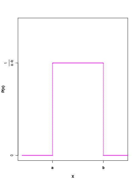
The plot of the Uniform distribution
The figure below displays the probability distribution function of a uniform distribution in the range \(\small{[a,b]}\). The function has a value \(\small{\dfrac{1}{b-a}}\) in the range \(\small{a \leq x \leq b}\) and is zero outside the region. This curve thus looks like a "step function".
The mean and variance of the Uniform distribution are obtained by,
Uniform random deviates
When a random variable \(\small{x}\) is drawn from a uniform distribution in an interval \(\small{[a,b] }\), the probability that its value lies in a small width \(\small{dx}\) inside the range is proportional to the width itself. Thus the probability that a random sample has a value in the range \(\small{[a,x]}\) is given by \(\small{\dfrac{x-a}{b-a}}\). When \(\small{a=0}\) and \(\small{b=1}\), we consider a distribution of x which takes values uniformly between 0 and 1. In computers, there are algorithms that can generate a large sequence of random numbers between 0 and 1. For a given input integer called "seed", a fixed sequence is generated by these algorithms. Every time we give a particular seed, we get the same sequence of random numbers between 0 and 1. Though a fixed sequence is generated for a seed, the numbers are random in a sense that given any number in the sequence, no algorithm or rule can predict what could be the next number or the previous number. The sequence is given, but the relationship between numbers in the sequence is totally random!. This sequence of n uniform random numbers are as good as sampling n numbers from a uniform distribution between 0 and 1. Knowing the sequence helps in repeating the random simulations. These random sequences are called pseudo random numbers as against real random numbers that are never reprodicuble in a sequence. Examples for real random numbers are the numbers generated by coin toss, converting random white noice from electrical circuits, thunder etc into numbers.
R scripts
R provides functions for computing uniform distribution with density f(x) = 1/(max-min)

 dunif(x, min=0, max=1) --------------> returns the uniform probability density
                                       in the range [min,max] for a given x value

 punif(x, min=0, max=1) --------------> returns the cumulative probability upto
                                       a given x value from min in the range [min, max].


 qunif(p, min=0, max=1) ---------------> returns the  x value at which the cumulative
                                       probability is p

 runif(n, min=0, max=1) ---------------> returns n random numbers in the range [min,max] from
                                        a uniform distribution.


In all the functions shown above, the default range is [0,1]

The R script below demonstrates the usage of the above mentioned functions:
##### Using R library functions for Poisson distribution

## Generate 5 uniform random numbers between 0 and 1.
x = runif(5)
format(x, digits=4)
print("five random numbers in [0,1] : ")
print(x)

print("")

## Generate 5 uniform deviates between 50 and 100
x = runif(5, min=50, max=100)
format(x, digits=4)
print("five random numbers in [50,100] : ")
print(x)

## Generate 100000 uniform deviates and plot the histogram
x = runif(100000)
hist(x, xlab="Value of random deviate x", ylab="Frequency", font.lab=2,
            breaks=10, main="", ylim=c(0,12000))
Executing the script creates the following output and the plot on the screen. As expected, the histogram of the uniform deviate has (almost) equal number of events in each bin between [0,1] for a very large number of events.
[1] "five random numbers in [0,1] : "
[1] 0.36261975 0.06758791 0.67829135 0.37133882 0.00848061
[1] ""
[1] "five random numbers in [50,100] : "
[1] 76.84919 94.26405 62.13572 88.91159 66.90542
