CountBio
Mathematical tools for natural sciences
Biostatistics with R
3D Histograms
The data for 3D histogram consists of a (X,Y) grid with n values of X and m values of Y. For each one of the $n \times m$ points on the grid, there is a Z value which is represented by a vertical column whose height is proportional to Z.
The
A list of important arguments to the
 x,y  ------> numeric vectors with m values of X and n values of Y

 z  ------> numeric matrix of dimension $m \times n$.


 theta, phi  -----> the azimuthal and colattitude directions for viewing. Angles in degrees.


 lighting ----->  If TRUE, the facets will be illuminated.
     Other values for this parameter are : "ambient", "diffuse", "specular", "exponent" etc.

 shade -----> Degree of shading of the surface. Value close to 1
              gives a shade similar to point light source, and values close to 0 produce
                no shading effect. Values between 0.5-0.75 approximates a day light.


space -----> amount of space as a fraction of bar width between bars.
                  Takes a value between [0,0.9]. Default is 0.

 label -----> A value of TRUE enables the label for axes.

 nticks -----> An integer specifying the number of ticks on the 3 axes.

 xlab, ylab, zlab -----> strings specifying labels for the three axes.

For other parameters of this function, type  help(hist3D) in R prompt.
Here is an example script for 3D histogram. We generate Y values between 1 and 13 on the X,Y grid using uniform random number generator. The function call runif(n*n, 1, 30) returns a vector of uniform random numbers between 1 and 30.
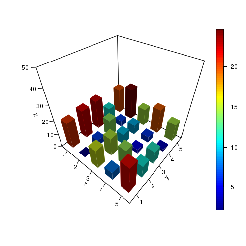
library(plot3D)

# X,Y and Z values
x = c(1,2,3,4,5)
y = c(1,2,3,4,5)

zval = c(20.8, 22.3, 22.7, 11.1, 20.1,
      2.2,  6.7,  14.1, 6.6,  24.7,
      15.7, 15.1, 9.9,  9.3,  14.7,
      8.0,  14.3, 5.1,  6.5,  19.7,
      21.9, 11.2, 11.6, 3.9,  14.8 )

# Convert Z values into a matrix.
z = matrix(zval, nrow=5, ncol=5, byrow=TRUE)


hist3D(x,y,z, zlim=c(0,50), theta=40, phi=40, axes=TRUE,label=TRUE, nticks=5,
        ticktype="detailed", space=0.5, lighting=TRUE, light="diffuse", shade=0.5)
The resulting scatter plot is shown below: