CountBio
Mathematical tools for natural sciences
Biostatistics with R
3D surface plots
Given the Z height values on a (X,Y) grid, we can draw the perspective plots of this surface over the (X,Y) plane. There are many options available in R for this. We will learn about the
Both these functions take almost similar set of parameters as arguments. We list some of the important ones here:
x,y ------> locations of grid lines at which values of z are measured. z ------> numeric matrix of dimension equal to number of grid points. Dimension of z = length(x) * length(y) theta, phi -----> the azimuthal and colattitude directions for viewing. Angles in degrees. scale --------> If scale is TRUE the x, y and z coordinates are transformed separately for viewing in the interval [0,1]. If scale is FALSE, the coordinates are scaled so that the aspect ratios are retained. Default is TRUE. shade -----> Degree of shading of the surface. Value close to 1 gives a shade similar to point light source, and values close to 0 produce no shading effect. Values between 0.5-0.75 approximates a day light. box -----> a default value of TRUE renders the bounding box. label -----> A value of TRUE enables the label for axes. nticks -----> An integer specifying the number of ticks on the 3 axes. xlab, ylab, zlab -----> strings specifying labels for the three axes. For other parameters of this function, typehelp(persp) orhelp(persp3D) in R prompt. For other parameters of this function, typehelp(scatter3D) in R prompt.
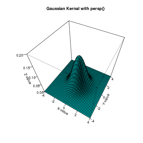
In order to create an impressive surface plot, we generate data using 2D Gaussian kernal expression. For independent variables (x,y), this formula generates y coordinates on a 2D Gaussian surface.
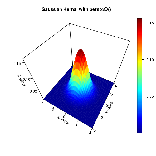
In the code given below, we first generate (x,y,z) coordinates of the surface. We then call the two functions persp() and persp3D() separately to create surface plots for the data. The two plots will be generated on separate canvas on the terminal. The plots are given in the end.
##  2D Gaussian Kernal plot

## Generate x and y coordinates as sequences
x = seq(-4,4,0.2)
y = seq(-4,4,0.2)

# An empty matrix z
z = matrix(data=NA, nrow=length(x), ncol=length(x))

### Gaussian kernal generation to fill the z matrix.
sigma = 1.0
mux = 0.0
muy = 0.0
A = 1.0

for(i in 1:length(x))
{
  for(j in 1:length(y))
  {

z[i,j] = A * (1/(2*pi*sigma^2)) * exp( -((x[i]-mux)^2 + (y[j]-muy)^2)/(2*sigma^2))
  }
}

### Now z is a matrix of dimension length(x) * length(y)

# Plotting surface with persp() function of default "Graphics" library in R.
## (Note: At this point, just give any x,y vector and z matrix of terrain to
##       get your plot)

persp(x,y,z, theta=30, phi=50, r=2, shade=0.4, axes=TRUE,scale=TRUE, box=TRUE,

      nticks=5, ticktype="detailed", zlim = c(0,0.2) , col="cyan", xlab="X-value",

      ylab="Y-value", zlab="Z-value", main="Gaussian Kernal with persp()")

##--------------------------------------------------------


## Create next plot on a separate canvas.
X11()


# Required for using persp3D() function below.
library(plot3D)


## We call persp3D function for same Gaussian kernal data generated above.

persp3D(x,y,z,theta=30, phi=50, axes=TRUE,scale=2, box=TRUE, nticks=5,

        ticktype="detailed", xlab="X-value", ylab="Y-value", zlab="Z-value",

        main="Gaussian Kernal with persp3D()")
The resulting surface plots are shown below: